Simple RAG: The Foundation of Document-Powered AI

Teaching a language model to look things up before answering, instead of guessing from memory.

Prerequisites: Basic understanding of what a language model (LLM) does. Familiarity with the idea of a database.

The Problem

Imagine you have a 200-page report about climate change. You need a quick answer: “What does chapter 2 say about the main cause of climate change?” So you ask a language model.

The model gives you a generic, textbook-style answer about greenhouse gases. It sounds reasonable. But it is not drawn from your report. The model has never seen your document. It is answering from memory, from patterns learned during training. It might even state facts that sound right but are nowhere in your source material. This is called hallucination, and it is one of the biggest risks of using language models for knowledge work.

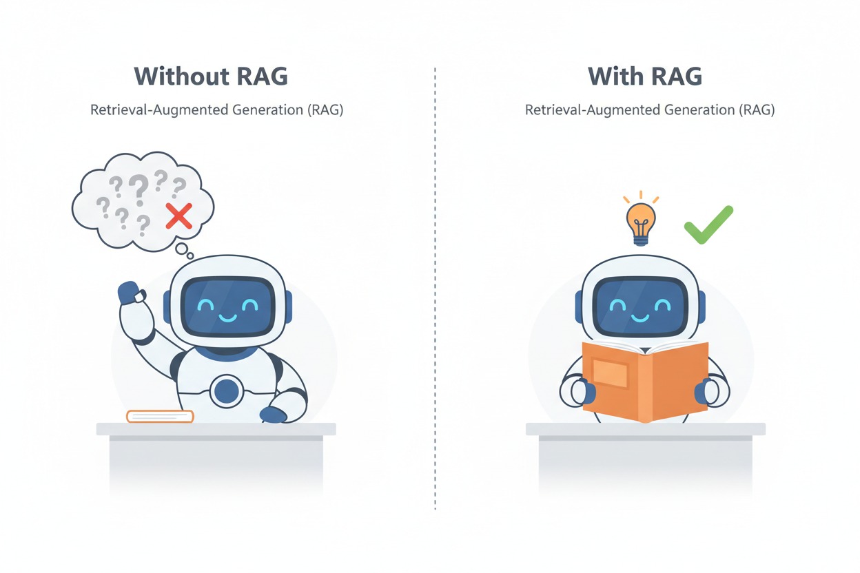
Now scale this up. Your company has thousands of internal documents: policy manuals, research papers, product specs, legal contracts. Employees ask questions about these every day. A language model that answers from memory alone is useless here. It does not know what is in your documents. The contrast is stark: without access to your documents, the model guesses and often gets it wrong. With access, it reads the relevant passage and answers correctly. The following illustration captures this difference.

The Core Idea

RAG, short for Retrieval-Augmented Generation, solves this by adding a simple step: before the model answers, it first searches your documents for relevant information.

Think of it as the difference between a closed-book exam and an open-book exam. In a closed-book exam, the student relies entirely on memory, staring at the blank page with growing uncertainty. In an open-book exam, the student can look up the relevant section, read it, and write an informed answer with confidence. RAG gives your language model an open book.

The core insight: you do not need to retrain the model or stuff entire documents into the prompt. You store your documents in a searchable format, retrieve only the relevant pieces, and hand those pieces to the model as context.

The model does what it does best: read the context and generate a clear, grounded answer. The rest of this chapter explains exactly how this works, step by step.

How It Works

The simple RAG pipeline has two phases: an offline preparation phase (done once per document) and an online query phase (done each time a user asks a question).

Phase 1: Preparing the Knowledge Base

Step 1: Load the Document

The process starts by extracting raw text from your source documents. A PDF is parsed page by page, converting visual content into plain text. This is a straightforward conversion step, but it matters. Poor text extraction leads to poor retrieval downstream.

Think of this as a librarian transcribing a book onto index cards so it can be cataloged and searched.

Step 2: Split Into Chunks

A 200-page document is far too large to search as a single block. The system splits the text into smaller pieces called chunks. A common default is chunks of about 1,000 characters (roughly a long paragraph), with 200 characters of overlap between consecutive chunks.

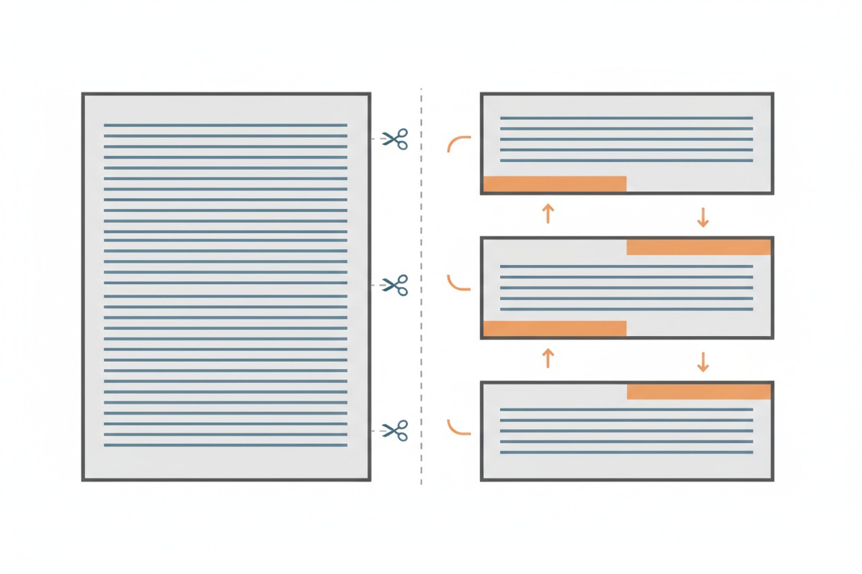
Why overlap? Imagine a critical explanation that spans two paragraphs. If you split the text exactly between them, neither chunk captures the full thought. The overlap ensures that information at the boundaries is preserved. Each chunk carries the last few lines of the previous chunk and the first few lines of the next one, so no thought is lost at the seams. The diagram below shows this: notice how the orange-highlighted bands at the bottom of one chunk match the top of the next, representing the shared overlap region.

Step 3: Clean the Text

Raw text extracted from PDFs often carries formatting artifacts: stray tab characters, extra whitespace, broken line endings. A cleaning step normalizes the text so that the next stages work reliably. This is a small but important detail. Dirty text leads to noisy embeddings.

Step 4: Create Embeddings

This is the most important transformation in the pipeline. Each text chunk is converted into an embedding: a list of numbers (a vector) that captures the meaning of the text. These are not random numbers. They are carefully computed so that two chunks about similar topics produce vectors that are close together in mathematical space, while chunks about different topics produce vectors that are far apart.

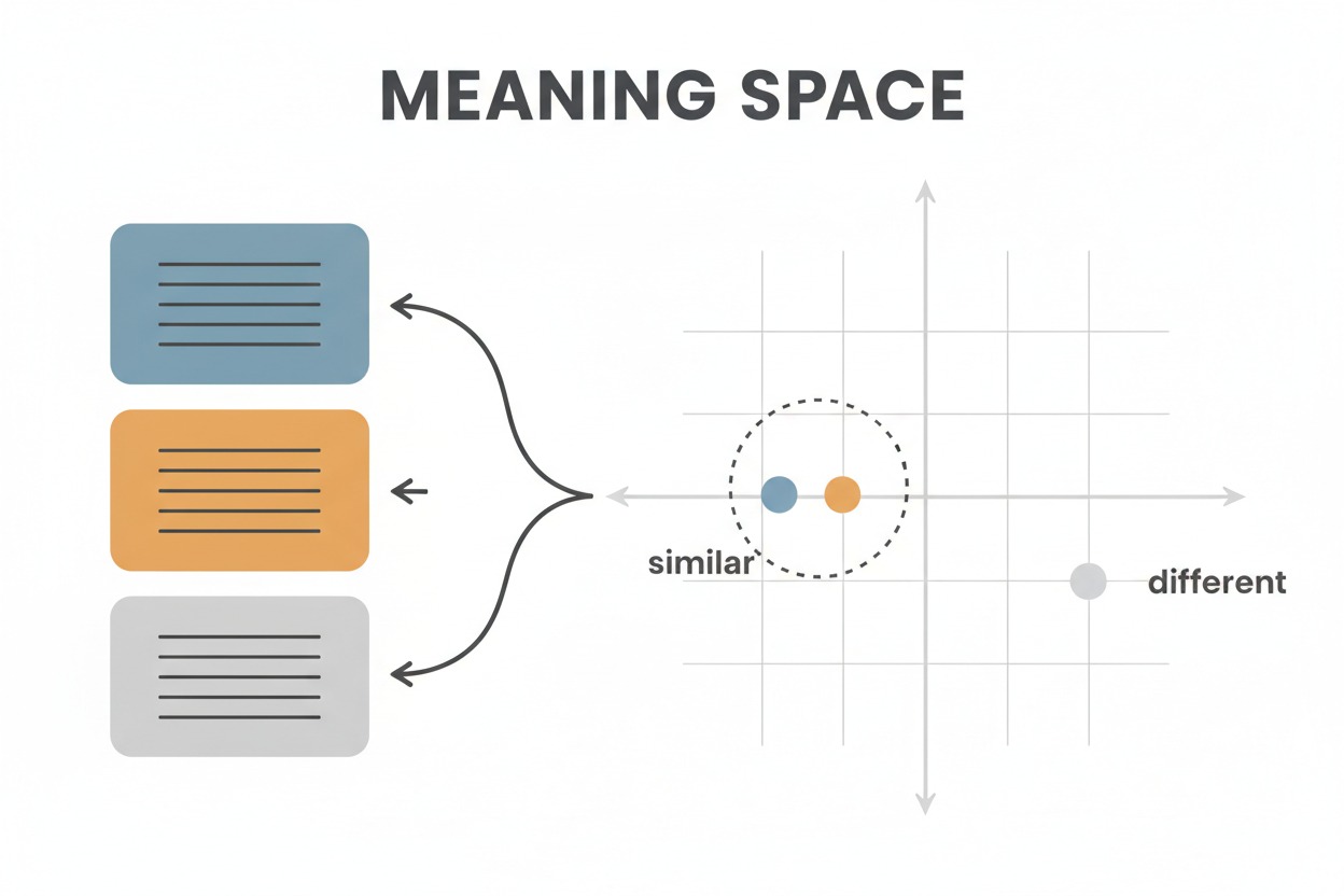
Think of embeddings as GPS coordinates for meaning. Just as GPS coordinates let you find places that are geographically close, embedding vectors let you find text passages that are semantically close. A chunk about “greenhouse gas emissions” and a chunk about “carbon dioxide in the atmosphere” will have nearby vectors, even though they use different words. The illustration below shows this: the blue and orange text cards map to dots that cluster together (labeled “similar”) because they cover related topics, while the gray card maps to a distant dot (labeled “different”).

Step 5: Store in a Vector Database

All embedding vectors are stored in a specialized database optimized for similarity search. A popular choice is FAISS (Facebook AI Similarity Search), which organizes vectors so that finding the nearest neighbors to any query vector is extremely fast, even with millions of entries.

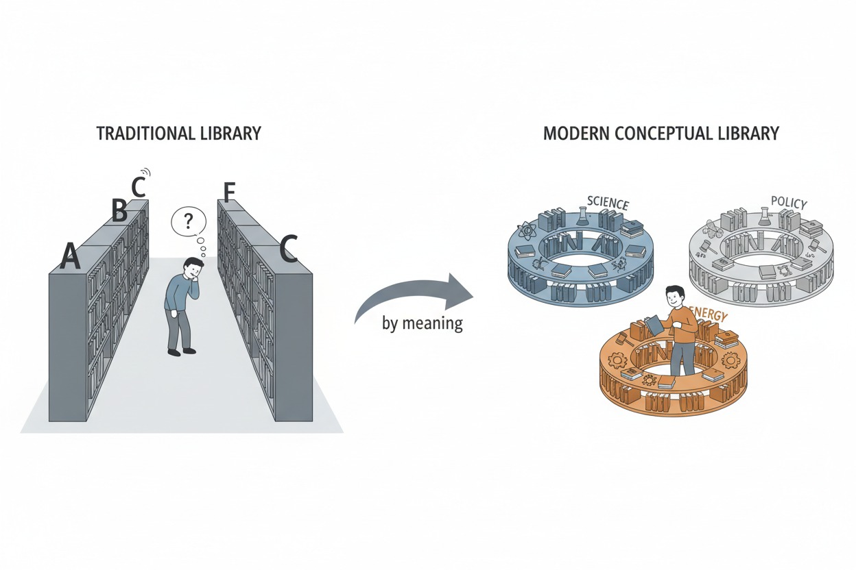
This is like organizing a library not alphabetically or by publication date, but by topic similarity. Books about related subjects sit on adjacent shelves. When you need information about a specific topic, you go straight to the right neighborhood and browse nearby books. The image below illustrates this contrast: a traditional library where a reader walks between distant shelves to find related books, versus a conceptual library where books on science, energy, and policy are clustered by meaning, putting relevant material within arm’s reach.

The entire preparation phase can be summarized in five steps:

Algorithm Sketch: Document Preparation

1. Load document and extract raw text
2. Split text into chunks of ~1000 characters with ~200 character overlap
3. Clean each chunk (remove formatting artifacts)
4. Convert each chunk into an embedding vector
5. Store all vectors in a vector store for fast similarity search

Phase 2: Answering a Query

With the knowledge base prepared, the system is ready to answer questions. This phase runs every time a user submits a query.

Step 6: Embed the Query

When a user asks a question, that question is converted into an embedding vector using the exact same process applied to the document chunks. This is critical: the query must live in the same “meaning space” as the stored chunks so that distances between them are meaningful.

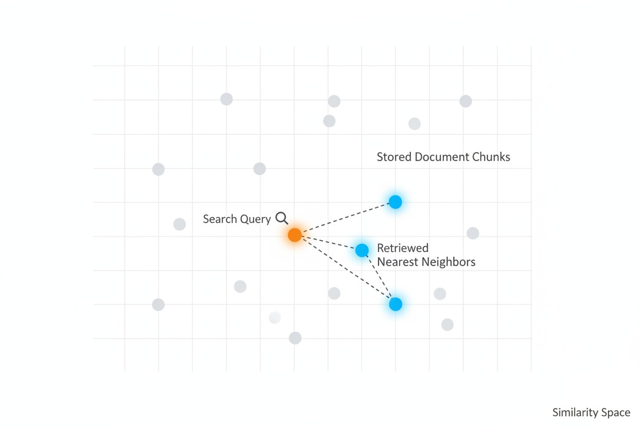
Step 7: Find the Nearest Chunks

The system searches the vector store for the chunks whose embedding vectors are closest to the query vector. A typical setup retrieves the top 2 to 5 most similar chunks. These represent the parts of the document most likely to contain the answer.

For example, given the query “What is the main cause of climate change?” against a climate report, the system might retrieve a chunk discussing greenhouse gases and fossil fuels, and another covering modern scientific observations about human-driven climate change. Both are directly relevant to the question. In the diagram below, the orange dot represents the query in meaning space, and the blue highlighted dots are the nearest stored chunks that the system retrieves, connected by dashed lines to show proximity.

Step 8: Generate the Answer

The retrieved chunks are passed to the language model along with the original question. The model reads the relevant context and generates an answer that is grounded in the actual document content, not in its training memory. This is the payoff. The model is no longer guessing. It is reading the relevant paragraphs and summarizing them for you.

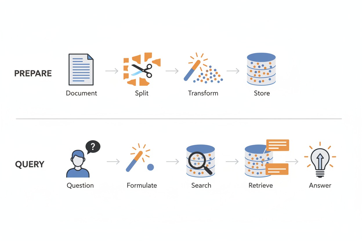
The diagram below shows the complete pipeline end-to-end. The top row is the preparation phase: a document is split, transformed into vectors, and stored. The bottom row is the query phase: a question is formulated into a vector, used to search the database, and the retrieved chunks feed into the final answer.

Algorithm Sketch: Query Processing

1. Receive user question
2. Convert question into an embedding vector
3. Search vector store for top-K nearest chunk vectors
4. Retrieve the corresponding text chunks
5. Pass question + retrieved chunks to the language model
6. Model generates answer grounded in the retrieved context

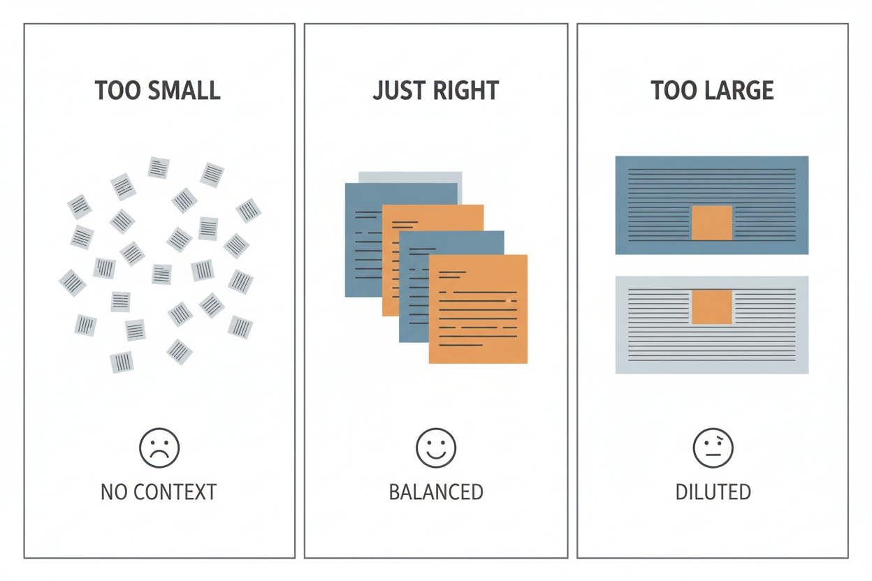
The Role of Chunk Size

Chunk size is the most important configuration decision in simple RAG, and there is no single right answer. It is a tradeoff:

Too small (e.g., 100 characters): Each chunk is just a sentence or two. It may be very specific, but it lacks surrounding context. The model gets a precise fragment but cannot understand the bigger picture.

Too large (e.g., 5,000 characters): Each chunk covers several pages. The relevant information is buried in a sea of unrelated text. The retrieval still works, but the signal is diluted by noise.

Just right (e.g., 1,000 characters with 200 overlap): Each chunk is roughly a full paragraph. It carries enough context to be meaningful on its own, but is focused enough to rank well in similarity search. The three panels below show this visually: tiny scattered fragments with no context, balanced medium-sized pieces, and oversized blocks where the relevant text is a tiny fraction of the whole.

Where Simple RAG Falls Short

Simple RAG handles focused, factual questions well. Ask “What is the main cause of climate change?” and the system retrieves the right paragraphs and produces an accurate, grounded answer.

But consider a harder question: “Compare the economic impacts of climate change across different sectors discussed in the report.” This requires information scattered across multiple sections of the document. A system that retrieves only two or three chunks will miss most of the relevant material. The answer will be incomplete or shallow.

Similarly, questions that require reasoning across multiple concepts, synthesizing definitions, or connecting ideas from different parts of a document will expose the limits of retrieving a small, fixed number of chunks from a single search.

These limitations are not bugs. They are the natural boundaries of the simplest possible RAG design. They are also exactly what motivate the advanced techniques covered in later chapters: better chunking strategies, multi-query retrieval, reranking, and query transformation.

When to Use This

Best for:

• Answering factual questions about a single document or small collection
• Building a quick prototype to validate that RAG helps your use case
• Internal knowledge bases with straightforward lookup queries
• Situations where simplicity and low cost matter more than perfect accuracy

Overkill when:

• Your documents are short enough to fit entirely in the model’s context window
• You only need keyword search (traditional search engines work fine)
• You never update your document collection and could pre-compute all answers

Tradeoffs:

Factor	Impact
Latency	Low: one embedding call + one vector search + one LLM call
Complexity	Low: fewest moving parts of any RAG approach
Cost	Low: embedding is cheap, only one LLM call per query
Accuracy gain	Moderate: strong for focused factual queries, weak for multi-hop or complex questions

Compared to using an LLM without RAG: Simple RAG grounds the model’s answers in your actual documents, reducing hallucination and enabling responses about content the model never saw during training. The tradeoff is that answer quality depends entirely on retrieval quality. If the wrong chunks are retrieved, the answer will be wrong or incomplete. And with a fixed chunk size and a single retrieval strategy, simple RAG has limited ability to handle nuanced or multi-part questions.

---

Key Takeaways

• RAG adds a “look it up” step before the language model answers, grounding responses in actual source material instead of training memory.
• Documents are split into overlapping chunks to ensure no information is lost at the boundaries between pieces.
• Embeddings convert text into numerical vectors where similar meanings are placed close together, enabling search by meaning rather than keywords.
• A vector store organizes these vectors for fast similarity search, even across millions of chunks.
• Simple RAG is the foundation that all advanced techniques build upon. Its limitations, including fixed chunk sizes, single-strategy retrieval, and no query refinement, are exactly what the rest of this book addresses.

Companion Notebook

The working implementation of this technique is in simple_rag.ipynb in the RAG Techniques repository.